During this regular season, I took on the challenge of creating an NBA MVP-related regression model given independent variables, like points per 36, assists per 36, & team wins, to attempt to assess a voting process and therefore predict future winners given voting history. But for the 3rd year in 11 seasons, the model’s projected voting tally & the true result featured some dissonance.
Foiled again!
Russell Westbrook took home NBA MVP honors and exceeded the Steadylosing MVP Model’s choice, James Harden, by a country mile. Could it be that the voters were enthralled by triple-double fever and hyperbolized the extent to which Russell’s teammates weren’t great (Bruce Bowen called OKC’s ancillary pieces “high school players” in one interview)? Did voters underestimate the extent to which Houston’s offense was elite? (As far as offenses are ranked, ’17 Houston appears somewhat legendary — 44th all-time when adjusting for league-wide efficiency.) Maybe, but Russell Westbrook was indefatigable & pretty fantastic, all things considered. The late spike in his team’s win pace easily elevated his reputation with voters and even gave his MVP bid greater favor in an analytical environment.
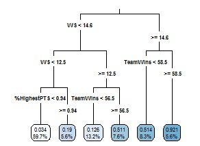
Take a quick look at how this regression tree explains that fulfilling certain criteria can affect the share of MVP points that you can acquire. It appears that winning greater than 58-59 games with significant production will make an MVP a fait accompli.
Although Westbrook didn’t gather the team win tally that would’ve made his victory assured, you can see how it’s beneficial to pick up wins and fall into the favor of the voters.
Here’s how to interpret the schematic:
There are 144 initial observations before any splits.
The first set of tree branches divides the database based on whether the player’s Win Shares are over/under the threshold of 14.6.
Because Stephen Curry had 17.87 Win Shares in 2015-16, he would separate toward the right of the diagram along with 19 other members.
Any player who doesn’t meet this requirement can likely only reach a maximum of .511 share of the max MVP points.
If any player accounts for fewer than 14.6 Win Shares, then he will then have to pass through the next branch which is 12.5 Win Shares.
Draymond Green had 11.1 Win Shares this past season; therefore, he will move to the left of this individual branch with 94 others.
Otherwise, he’ll proceed to the right of the branch to the next iteration.
And so on…
Then, to show with which type of leaf (or, terminal node) each MVP candidate aligns:
Ultimately, we can’t escape the narratives that develop during the season. If a player is particularly charismatic, it’ll only help his candidacy. When seemingly insurmountable leads vanish and impractical comebacks culminate with climactic game-winners, we remember. If you were to give an MVP-caliber season a eulogy, you’d point to moments such as this.
ICYMI: Russell Westbrook broke the single-season triple-double record. Hit a monster game-winner in Denver. Unreal. pic.twitter.com/4nrmfxAfpz
— Up The Thunder (@UpTheThunder) April 10, 2017
(via Up The Thunder)
My previous model didn’t account for such standout performances, so I wanted to revisit & suggest some new independent variables that could give SteadyLosing MVP model remake even more explanatory power.
New Potential Variables:
- Max Scoring Output/Frequency of 40+ Point Outings – Box score statistics tend to jump out at us. Whenever a player scores in bunches with notable frequency his holistic impact might even be overvalued.
- Pythagorean Differential – This one is fairly simple: Pyth Diff = Team Wins – Pythagorean Win Projection. Therefore, if a player’s squad has a positive value, then he may be overachieving a bit or exceeding expectations by winning close games despite the suboptimal effort, which is truly beneficial to an MVP portfolio. In 2015-16, when the Golden State Warriors won 73 games, their Pythagorean Win Projection was only 65 games. This past season, Oklahoma City held a Pythagorean differential of (positive) four.
- Team Off/Def Efficiency Z-Scores – The extent to which a team is better at a side of the ball than other teams should carry a bit of significance. Many fans prefer offensive fireworks, so a team that measures more than a standard deviation above the mean (more than one z-score) will likely have a favorable reputation among voters.
- TS% – Not because it’s trendy, but because if you take a look at the previous model, I used three-point shooting percentage and free throw percentage separately. Compounding TS% and usage percentage and yielding a high value could indicate star players who tend to be very efficient with their scoring.
It’s certainly not uncommon to use statistical analysis to predict the outcomes of processes that are confronted with a bit of subjectivity. Let’s ascertain which factors have been important to MVP consideration from past seasons, determine whether voters are straying from the trend & find out whether solid rationale exists during outlier years.
I’ll remember these new ideas for the next iteration of a SteadyLosing NBA MVP model.